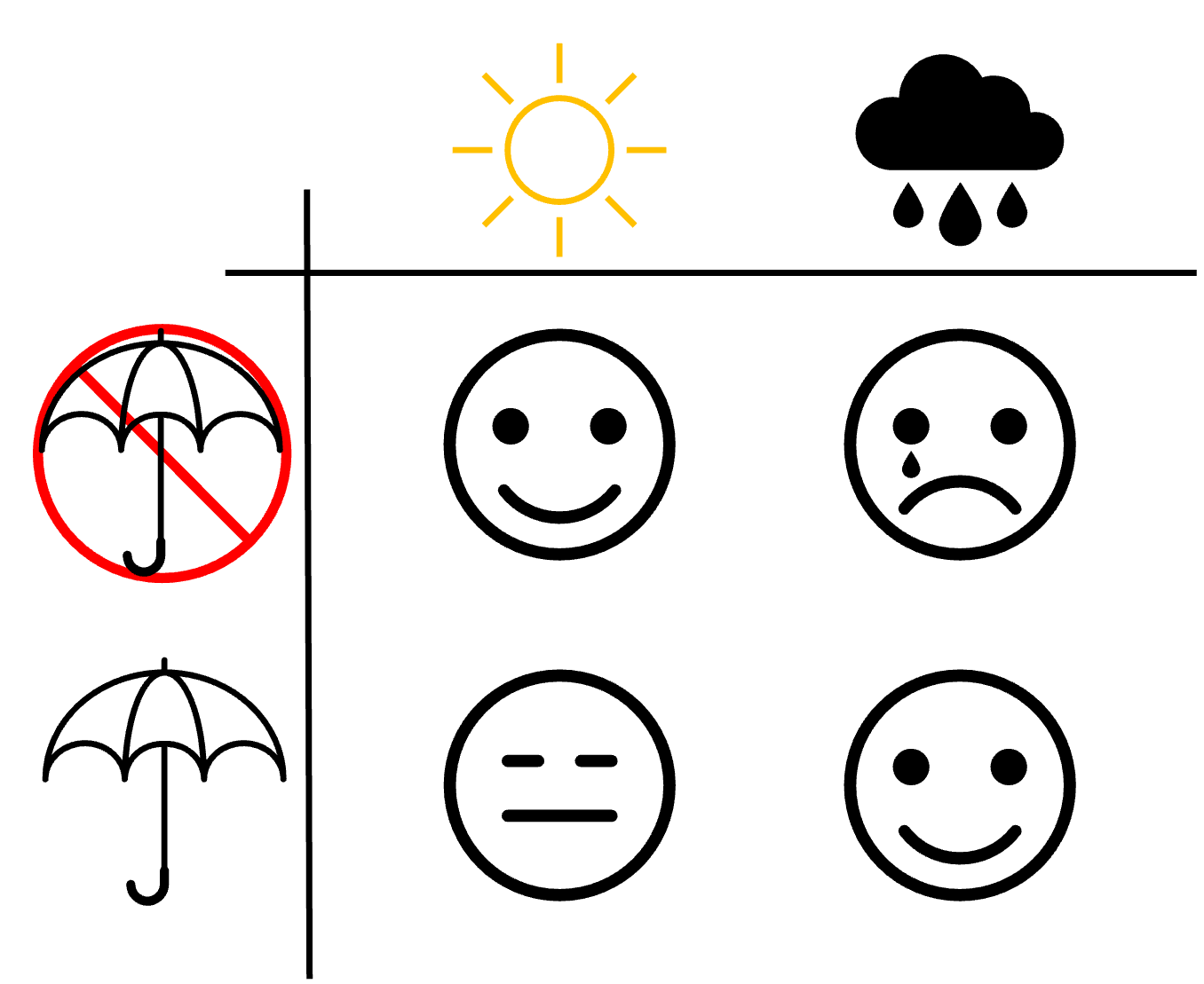
Every day we make decisions based on uncertain information. Living in the UK, a fantastic example of this is if you should take an umbrella with you. Weather forecasts are notorious. They can predict clear a blue sky and it ends up bucketing it down. That’s why most of the time I have an umbrella in my bag, just in case. Its a regret minimising decision, in other words, the cost of bring my umbrella with me and not needing it is much lower than needing it and not having it. Here is a fun picture to outline the possible states:

If we were to naively automate this system using a typical predict-then-optimise approach there would be two steps:

1. Create a rain prediction model that outputs a yes or no to if it will rain.
2. Create an optimisation process (in this case just a check to see if rain is predicted) to decide if I need an umbrella or not.

Im sure you can see a number of issues and some obvious ways to improve this approach. We could do more that just predict a binary variable, $p\in 0,1$, for if it will rain, we could predict a probability or how heavy the rain will be. Doing so would complicate our optimisation step, perhaps now we use a threshold value. However, this doesn’t address the underlying issue of, what if the prediction is wrong? The optimisation process as no knowledge its using predictions, and more importantly, the model has learned to minimise its prediction error ($L2$) with no regard for the optimisation. Unlike the predict-then-optimise approach, Decision-Focused Learning is the process of teaching machine learning models to generate predictions that when used to make a decision minimise regret.

The maths

Machine learning

The typical machine learning (ML) process is defined as follows. Given a set of pairs of features and labels: $\mathcal{D}=\{(x_1,y_1),(x_2,y_2)\dots (x_n,y_n)\}$ where $x_i$ is an $nd$ feature vector $x=[f_1,f_2\dots f_n]$ sampled from $X$ and its values have some correlation to $y_i$

Assuming that it exists, we want to learn the true function $\mathcal{F}(x_i)=y_i$. However, this isn’t possible, so we use the data, $D$, to learn a model $M$ where $M(x_i)\to \widehat{y_i}$ that minimises a loss function $\mathcal{l}$ between $y$ and $\hat{y}$. A typical loss function might look something like $l=(\widehat{y_i}-y_i{)}^2$. For a parametrised model the learning process looks like

$$\begin{array}{}\text{(1)}& {\theta }^{\ast }=\underset{\theta }{\mathrm{argmin}}\frac{1}{n}\sum _{i=0}^{n}l(y_i,M_{\theta }(x_i))\end{array}$$

where ${\theta }^{\ast }$ would be the optimal parameters for the model given the data available.

Optimisation

In a classical optimisation process, we attempt to find the optimal solution $z\ast$ to a problem. $z\ast$ is typically defined as being drawn from the set of all valid solutions $z\ast \in Z$. Though in some notation $Z$ can be the space of all possible solutions, valid or not and constraints are applied to the optimization process. We will use $Z$ for the valid solution space and $\mathcal{Z}$ for the larger space of all possible solutions. In math notation, $Z\in \mathcal{Z}s.t{g}_i(z)\le 0,\text{for}i\in \{1,\dots ,m\}\mathrm{\forall }z\in Z$ where $g$ is a constraint on the solution.

The optimality of a solution is measured using a fitness function $f$. We can define the optimisation process as

$$\begin{array}{}\text{(2)}& z^{\ast }=\underset{z\in Z}{\mathrm{argmin}}f(z)\end{array}$$

Of note here is that $f$ can often be computationally expressive or $Z$ so large it is infeasible to try all possible solutions. As such, methods must be used to reduce the search space to find the solution. This is typically a combination of heuristics (often defined using domain expertise) and advanced search methods such as genetic algorithms. In fact, the machine learning problem defined in [$\text{1}$] is an optimisation problem.

In the case of the ML problem with a parametrised model such as a neural network. It is possible to calculate gradients and use them to direct the exploration of the solution space in order to find a solution $\widehat{z^{\ast }}$ that is close to the true optimal solution i.e. $\widehat{z^{\ast }}\approx z^{\ast }$

Predict-then-Optimize

In the predict-them-optimize setting, the optimization process depends on some unknown values. To find the true optimal solution, the fitness function must be conditioned on the unknown values $y$. As such [$\text{2}$] must be reformulated to $z^{\ast }(y)={\mathrm{argmin}}_{z\in Z}f(z,y)$. In a practical sense, this is infeasible as $y$ is unknown. To circumvent this issue the model $M_{\theta }$ can be used as $x$ is available. Using $M_{\theta }$ we can generate a value $\hat{y}$ to be used in the optimisation.

$$\begin{array}{}\text{(3)}& \begin{array}{r}\widehat{z^{\ast }}(M_{\theta }(x))=\widehat{z^{\ast }}(\hat{y})=\underset{z\in Z}{\mathrm{argmin}}f(z,\hat{y})\end{array}\end{array}$$

We use the notation $\widehat{z^{\ast }}$ here to denote it is the optimal solution found using predictions of $y$. If the model perfectly reconstructs the true values of $y$ then the solution found should be the true optimal solution i.e. $\widehat{z^{\ast }}=z^{\ast }$.

Note that $dim(y)=D$ is typically high as all values needed to parametrise the optimisation problem are predicted. As such it is likely comprised of the output multiple models $\hat{y}=[\widehat{y_1},\dots ,\widehat{y_D}]=[M_{\theta }(x_1),\dots ,M_{\theta }(x_D)]$ where each model predicts an individual component e.g. travel time, supply, demand, and cost.

• Pros

This is simple to implement. Predictive models are fairly easy to learn. Can use any optimization method.

• Cons

No information about the optimization process is passed into the model.

It has been shown that model misspecification can lead to extreme errors when multiple correlated variables are combined in the optimization process [@Cameron2022]

Decision-Focused Learning

In the PTO setting, we noted that when $\hat{y}=y$, should result in a solution where $\widehat{z^{\ast }}=z^{\ast }$. However, models learned using [$\text{1}$] will almost always have some error. The error induced by sub-optimal solution $\widehat{z^{\ast }}$ selected by the fact that $\hat{y}\ne y$ is called the decision loss (DL). It is the value of the fitness function of the solution $\widehat{z^{\ast }}$ generated using predicted values, evaluated using the ground truth values of $y$.

$$\begin{array}{}\text{(4)}& DL(\hat{y},y)=f(\widehat{z^{\ast }}(\hat{y}),y)\end{array}$$

In a [DFL]{acronym-label=”DFL” acronym-form=”singular+short”} setting our goal is now reformulated. We aim to learn a model $M_{\theta }$ that minimises the [DL]{acronym-label=”DL” acronym-form=”singular+short”}. For the dataset $\mathcal{D}$, the learning process would be:

$$\begin{array}{}\text{(5)}& {\theta }^{\ast }=\underset{\theta }{\mathrm{argmin}}\frac{1}{n}\sum _{i=1}^{n}DL(M_{\theta }(x_i),y_i)\end{array}$$

• Pros Better performance.

• Cons

Hard to implement; Can be more computationally expensive to learn; Still have an (expensive) optimization step